Stochastic gradient descent to find least square in linear regression

Let’s go back to a very simple yet strong method we use in model: linear regression. As most of people know the way to fit linear regression is used least square or maximum likelihood function. Using least square as example, most of people has statistics background knowing that the estimators are: (x’x)-1(x’y). But how do the majority statistical software implement this algorithm? Normally they use QR decomposition.

QR decomposition:
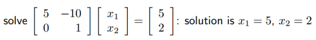
Suppose we want to fit the model: Y=Xb. We do a QR decomposition: X=QR. Here Q is a orthogonal matrix Q’=Q-1; R is a upper triangular matrix. X’Y=X’Xb. Using the rule that X=QR, we can get R’Q’Y=R’Q’QRb. since Q is a orthogonal matrix. Q’Q=I. Hence R’Q’Y=R’Rb -> Q’Y=Rb. since R is a upper triangle matrix, we can easily get results based on back substitution. One example of back substitution as follows:

QR decomposition is very good way because we don’t need to do matrix inverse any more. As we always know, matrix inverse requires a lot of computational powers to solve.

Stochastic gradient descent:
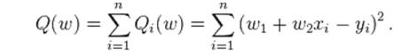
Stochastic gradient descent is an optimization method to find a optimal solutions by minimizing the objective function using iterative searching. Suppose we want to find optimal b, which can minimize square loss function, we can initially assign b0. Then b(t)=b(t-1)-a∇L(b). Here ∇L(b) is the partial derivative of loss function corresponding to b. Suppose we have y=h(x). For multiple regression, we can write in this way:

Normally, because the training dataset is very large, we use one random training sample each iteration to get optimal solution. The Stochastic gradient descent equation using one random training obs each time is:
 

If we use one random sample per iteration, we may get solution, which is not but close to the global optimal solution.

Stochastic gradient descent can also be useful for implementing parallel linear regression algorithm. (iterative reduce: YARN package).

Here I share some sample R codes for a simple linear regression case. For multiple linear regression, we can use the same algorithm but do a few changes there. One challenge to implement the algorithm is how to correctly setup the descent rate. If it is too large, the iteration may not be converged. If it is too small, it is too slow to get the final results.

#####code to implement Stochastic gradient descent in simple linear regression####
##Firstly get some dummy data###
x <- runif(1000000,1,100);
y <- 5+4*x;
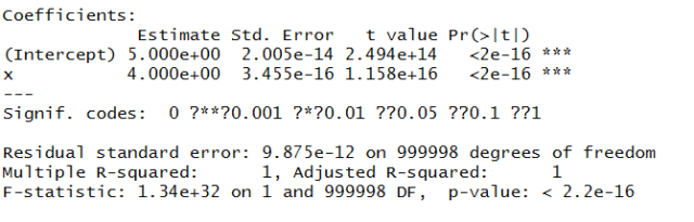
###do a least square###
fit <- lm(y ~ x);
summary(fit);
###do a Stochastic gradient descent####
sgd<-function(x,y,b0,n,alpha) #here b0 is initial beta n is iterative loop###
{
#beta<-as.matrix(cbind(rep(b0[1],n),rep(b0[2],n)));
beta2<-as.matrix(cbind(rep(b0[1],n),rep(b0[2],n))); #SGD using one random sample per iteration
for (i in 2:n)
{
m<-length(x);
# beta[i，1]<-beta[i-1,1]-(1/m)*alpha*sum(beta[i-1,1]+beta[i-1,2]*x-y);
# beta[i，2]<-beta[i-1,2]-(1/m)*alpha*sum(x*(beta[i-1,1]+beta[i-1,2]*x-y));

sample_num<-sample.int(m,1);
xx<-x[sample_num];
yy<-y[sample_num];
beta2[i，1]<-beta2[i-1,1]-alpha*(beta2[i-1,1]+beta2[i-1,2]*xx-yy);
beta2[i，2]<-beta2[i-1,2]-alpha*(xx*(beta2[i-1,1]+beta2[i-1,2]*xx-yy));

}
return(beta2);
}
b0<-c(0,0)
beta<-sgd(x,y,b0,1000000,0.00005);
plot(beta[1:1000000,1], col='red');
lines(beta[1:1000000,2],col='green');

Result:
1) QR decomposition (default method in R):

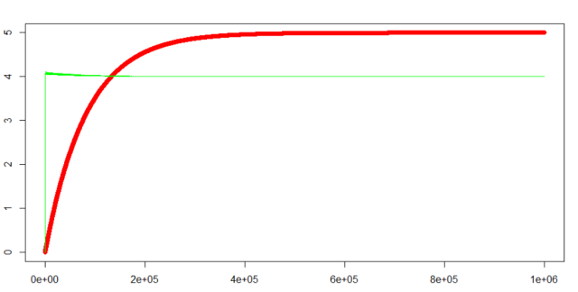
2) stochastic gradient descent result:

Red line is X1, green line is X2: